3 Tactics to Improve your Cluster Analysis

Clustering

Clustering is - at the same time - an intuitive algorithmic problem and a statistician’s nightmare.

From an algorithmic perspective, clustering is the task of dividing data points into groups (a.k.a. clusters) in such a way that points in any group are similar to each other, and every group is dissimilar to all other groups. Pretty straightforward. Although it is not necessarily straightforward to define what similar or dissimilar means.

From a statistical perspective, clustering raises some painful questions.

• What do clusters represent?

• Are these sample-level objects estimators for some characteristic of the population probability distribution that generated the data?

• If so, what characteristic are they estimating? And how do we assess our uncertainty around these estimates?

Modal clustering answers some of these questions and lends itself to a statistical interpretation of clustering for continuous variables under the assumption of well-behaved density functions. But a complete and unified statistical theory of clustering is hard to formulate.

Statistical theory aside, the algorithmic definition of clustering provided above also leaves room for very practical concerns.

Consider this: given any dataset, the cluster consisting of all points in the dataset is such that every point in this cluster is similar to all other points in the same cluster: all points in the dataset are part of the same dataset after all, so they are similar in this sense. Furthermore, this cluster is dissimilar to all other clusters: there are no other clusters!

Or this: given any dataset, each point in the dataset can be considered a cluster on its own. In fact, each point is similar to the points in the same cluster i.e., only itself. Each point is also dissimilar to the points corresponding to all other clusters: by definition, each unique point in a dataset is dissimilar to all other points.

Neither of the above extreme-case clustering structures is particularly useful in practice. Yet, they both satisfy the algorithmic definition of clustering. So, considering all possible clustering structures that we can generate from a dataset, how do we determine which ones are meaningful and which ones are not?

Unlike other Machine Learning (ML) tasks where we want to predict or classify some target variable using a set of predictors, there is no target variable in clustering. The lack of a target variable makes it a lot harder to evaluate whether a particular set of clusters that we found in a dataset is in any way meaningful. For regression tasks, we can evaluate the quality of a model in terms of Mean Squared Error (MSE). For classification tasks, we can compute metrics such as accuracy, precision, and recall. For clustering, we have essentially no way of measuring how far off we are from some “true” clustering structure that exists in the data.

Yet, cluster analysis is frequently performed in real-world applications (think customer segmentation in Marketing, for example). This is because - despite its difficulty - cluster analysis frequently leads to a better understanding of many datasets and produces useful business insights. But what are some of the tactics that we can use to improve our ability to discover meaningful clusters and be more confident about our discoveries? In the remainder of this post, we discuss 3 of them.

All code associated with this post is available in this GitHub repository.

Tactic 1: Algorithm Tuning

The running example in the remainder of this post is a Kaggle dataset containing information about 200 mall customers. Our goal is to evaluate whether we can find meaningful clusters of customers based on 3 variables: the customer’s age, the customer’s annual income (in thousands of dollars), and the customer’s spending score (between 1 and 100) assigned by the mall to each of the customers in the dataset. The customer’s gender is also available in this dataset, but we intentionally ignore it in this post to avoid dealing with a categorical variable and to keep the discussion simple. In a real-world setting, finding clusters of customers in this kind of dataset is relevant because it can lead to new marketing opportunities.

As a first step, we visualize the mall customers dataset with a pair plot.

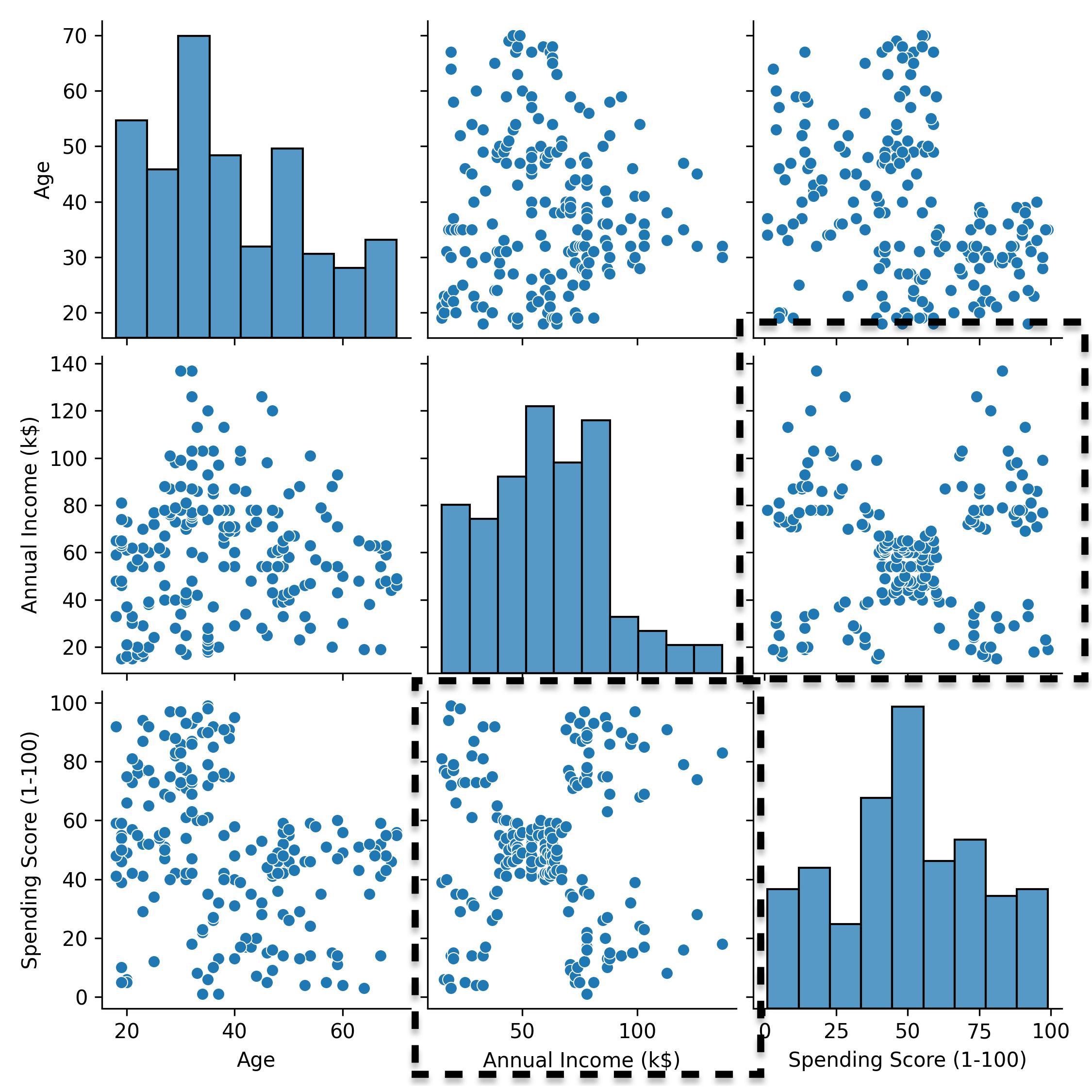
Pair plot of the mall customers dataset.

The pair plot allows us to visualize 2 variables at a time. From the scatter plot of spending score and annual income, we notice that there may be 5 clusters of customers. We can use the k-means algorithm to try and recover them.

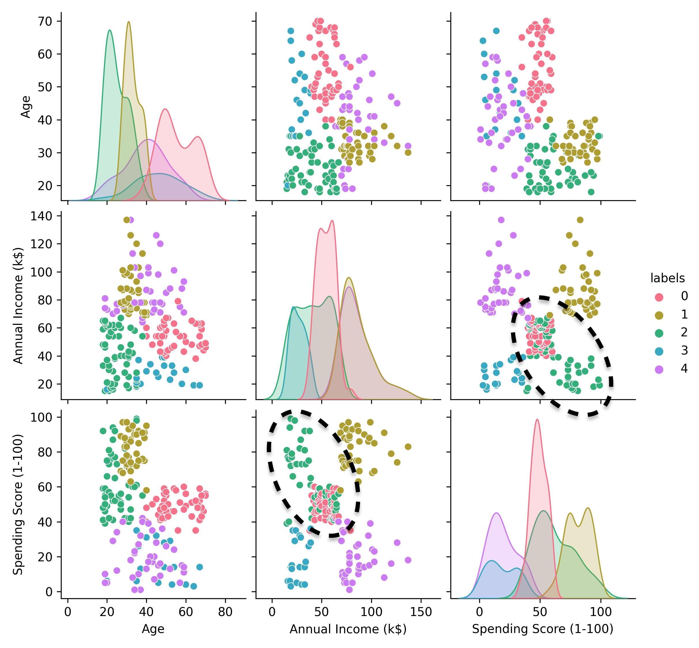
k-means clustering of the mall customers dataset (k=5).

The answer that we get from k-means is not exactly the one we expected. What we thought was an individual “central” cluster in the spending score and annual income scatter plot is instead - according to this k-means clustering - a group that is partially overlapping with a cluster of lower income, higher spending customers (cluster 2 in the pair plot).

This suggests that trusting our eyes may not be the best way to proceed. A better approach is to treat the number of clusters in the k-means algorithm as a tunable parameter. But how to tune a clustering algorithm like k-means?

We can tune a clustering algorithm by means of some sensible criterion. For instance, we could find the values of the tuning parameters of the algorithm that maximize some hand-crafted score function which captures our definition of what a good clustering structure is. Intuitively, a “good” clustering structure is one where the clusters are homogeneous within themselves (i.e., the points in any cluster are similar to the other points in the same cluster) and heterogeneous between them (i.e., the points in any cluster are dissimilar to the points in every other cluster). One such score function is the Silhouette score.

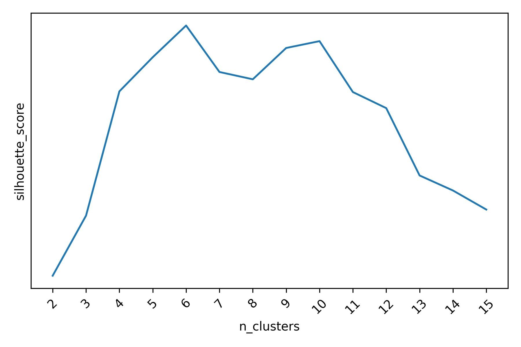
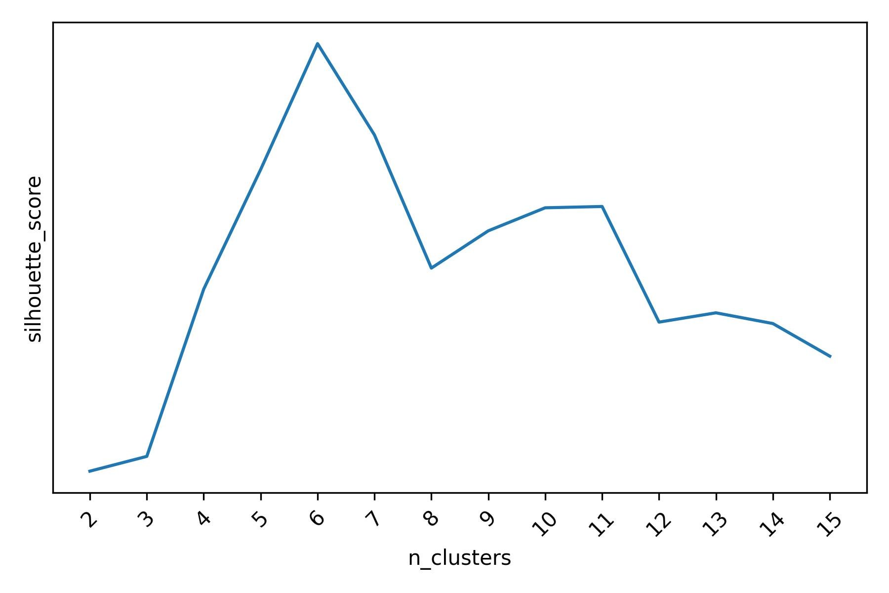
Silhouette score for different k-means clusterings of the mall customers dataset.

When evaluated using the Silhouette score, k-means indicates that there may be 6 or 10 clusters. The Silhouette score is in fact highest when k-means is asked to find 6 clusters, with another slightly lower peak at 10 clusters. When we visualize the 6 clusters obtained with k-means, we do observe a less ambiguous result.

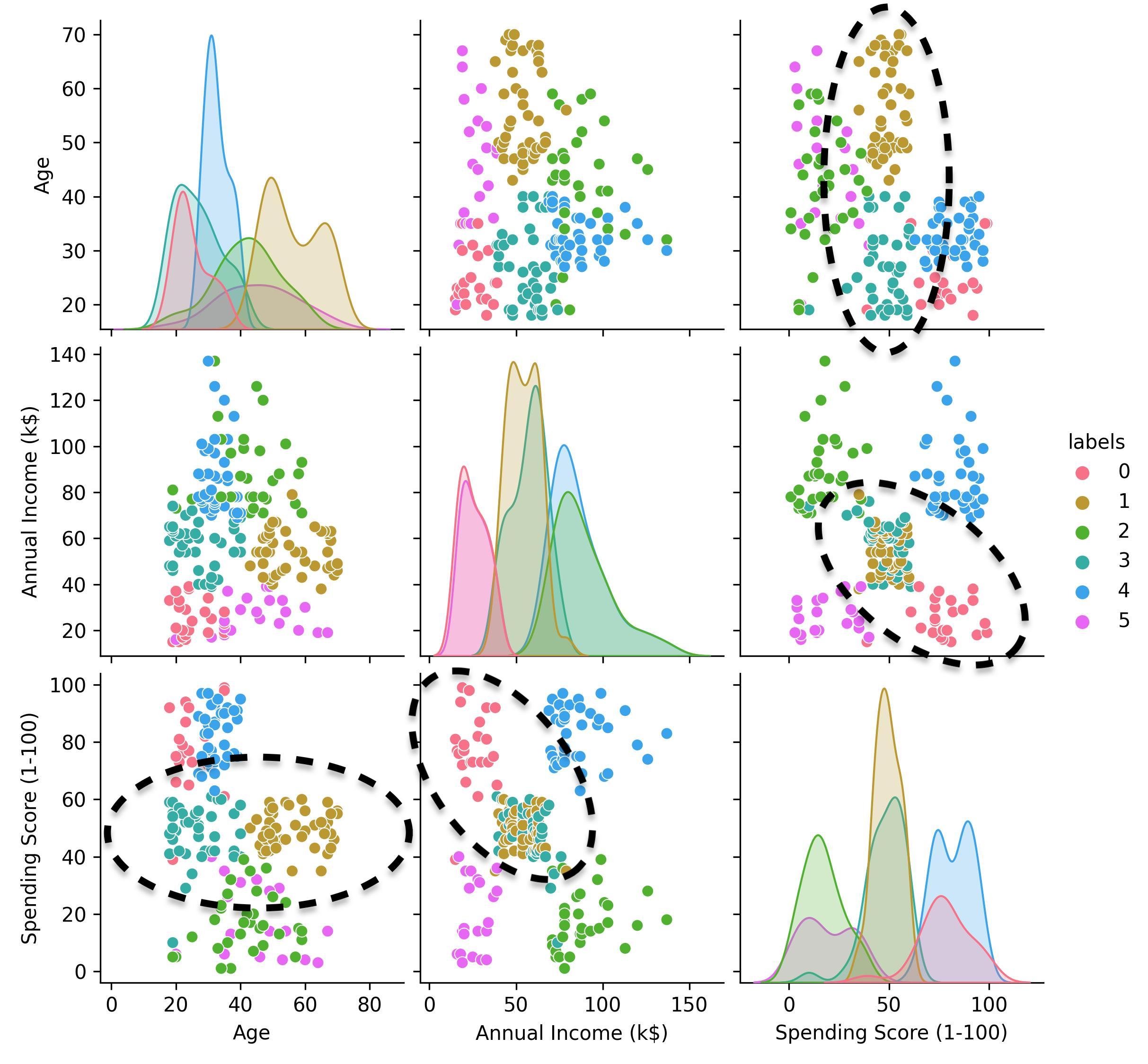
k-means clustering of the mall customers dataset (k=6).

The cluster of lower income, higher spending customers (i.e., cluster 0) is now well separated from the “central” group of points, which is still split into 2 clusters (clusters 1 and 3). The fact that clusters 1 and 3 are separated makes sense, since they consist of customers belonging to different age groups.

Running k-means with 10 clusters - the second-best parameter value according to the Silhouette score - produces a more granular clustering structure in which some of the 6 clusters are further split into 2 or 3 smaller clusters. The curious reader can verify this with the accompanying code.

With k-means, the tuning parameter is the number of clusters, which is very interpretable. However, the tactic that we just described can be applied to any tunable parameter(s) of any clustering algorithm.

By tuning a clustering algorithm using sensible scoring functions, we reach more solid conclusions. But how sensitive is the tuning procedure described above to the choice of the scoring function?

Tactic 2: Sensitivity Analysis

We used the Silhouette score to tune k-means to our data. However, the Silhouette score is only one way to capture our definition of what a good clustering structure should look like. In fact, other scoring functions such as the Calinski-Harabasz score or the Davies-Bouldin score also capture the same definition, but in different ways. It is therefore a good idea to evaluate how sensitive our tuning procedure is to the choice of the scoring function.

For this dataset, according to the Calinski-Harabasz score there may be 6 or 11 clusters when running k-means.

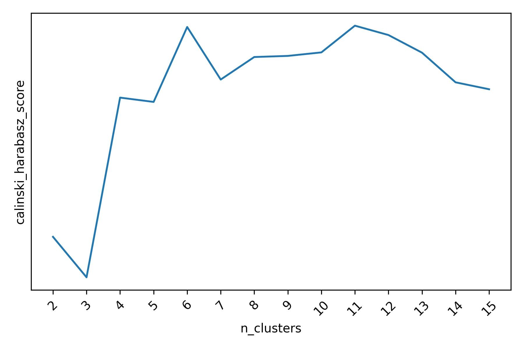
Calinski-Harabasz score for different k-means clusterings of the mall customers dataset.

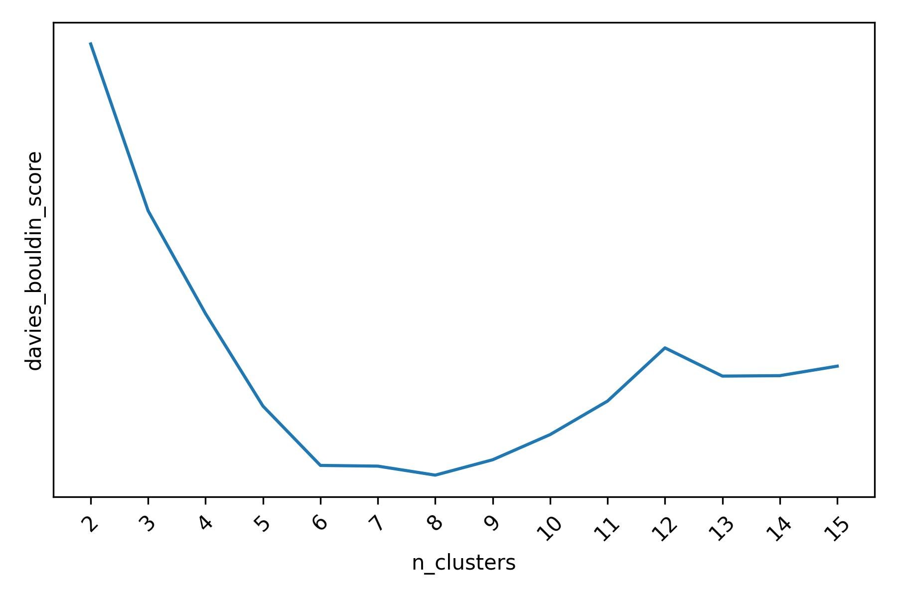
The Davies-Boulding score, similarly to the Silhouette score, indicates that there may be 6 or 10 clusters when running k-means (note that - unlike the Silhouette score or the Calinski-Harabasz score - lower values are better for the Davies-Boulding score).

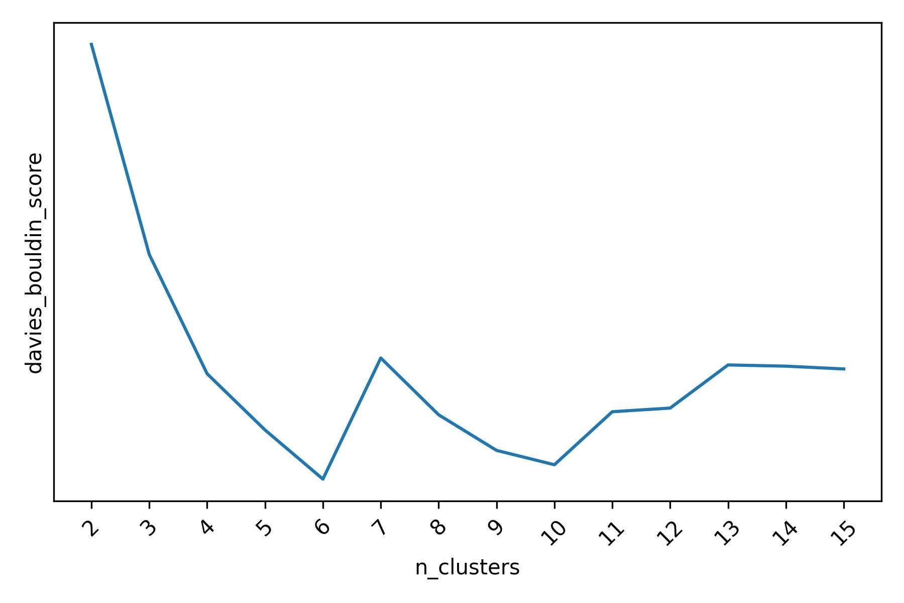
Davies-Bouldin score for different k-means clusterings of the mall customers dataset (lower values of the score are better).

Overall, it seems that all of the three scoring functions lead us to the same conclusion: there are 6 clusters of customers in this dataset, which could be further split into 10 or 11 smaller clusters.

By verifying that a clustering algorithm is not overly sensitive to the choice of the scoring function, we can partially rule out that the clustering structure that the algorithm found is simply a fluke in the tuning process. However, how would our conclusions change if we used a different clustering algorithm instead of k-means?

Tactic 3: Consensus Analysis

An additional step that we should take is to try and rule out that a particular clustering structure is detected only by a specific algorithm (e.g., k-means in our case). If we could replicate our findings with other clustering algorithms, we would be accumulating more substantial evidence about the fact that the clusters that we found represent some “real” characteristic of our data.

Agglomerative Clustering, confirms the presence of 6 clusters in our data when tuned with either the Silhouette score or the Calinski-Harabasz score.

Silhouette score for different Agglomerative Clustering clusterings of the mall customers dataset.

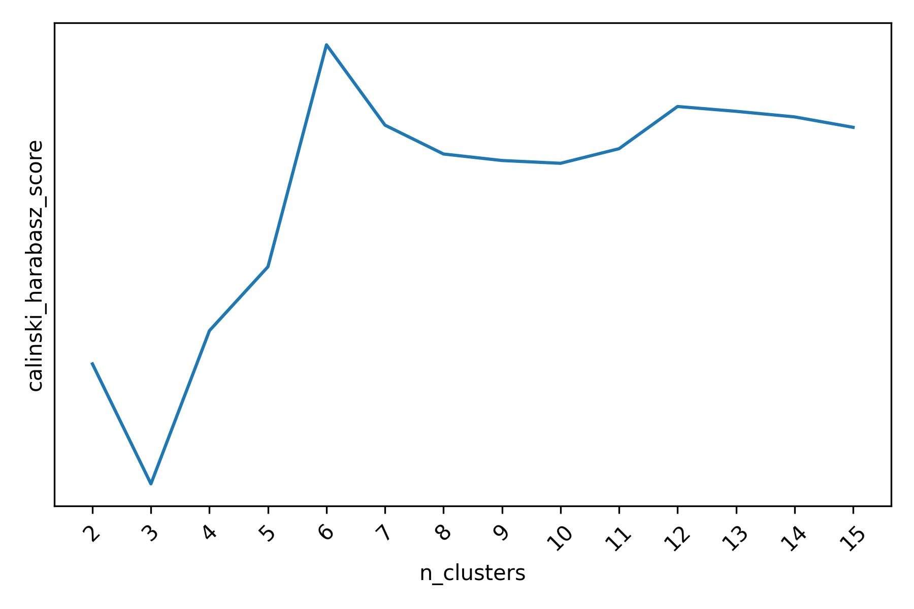
Calinski-Harabasz score for different Agglomerative Clustering clusterings of the mall customers dataset.

When using the Davies-Boulding score, we also see a strong indication that 6 clusters may be present (although 8 clusters is the best configuration according to this scoring function).

Davies-Bouldin score for different Agglomerative Clustering clusterings of the mall customers dataset (lower values of the score are better).

The fact that Agglomerative Clustering also hints at the presence of 6 clusters does not automatically imply that the 6 clusters are the same clusters that we previously found using k-means. This is something that we need to check.

When we compare the 6 clusters found by k-means and the 6 clusters found by Agglomerative Clustering, we observe a one-to-one correspondence between the two. To see this, we can use a cross-tabulation.

Cross-tabulation of clusters found using k-means with Silhouette score tuning and Agglomerative Clustering with Silhouette score tuning.

From the cross-tabulation above, we observe that cluster 0 of Agglomerative Clustering is the same as cluster 3 of k-means, cluster 1 of Agglomerative Clustering is the same as cluster 1 of k-means, cluster 2 of Agglomerative Clustering is the same as cluster 4 of k-means and so on.

It is useful to keep in mind that the cluster labels assigned by each algorithm are completely arbitrary: as long as we can find a one-to-one mapping between the cluster indices of one algorithm and the cluster indices of another algorithm - i.e., there are no or few off-diagonal elements after rearranging the rows or the columns of the cross-tabulation matrix - then the two algorithms are producing the same clusters. In fact, consensus between two algorithms can be found even in situations where the algorithms do not agree on the number of clusters (i.e., when the cross-tabulation matrix is not square). For instance, consider the cross-tabulation of the 6 clusters found by tuning k-means with the Silhouette score and the 8 clusters found by tuning Agglomerative Clustering with the Davies-Bouldin score.

Cross-tabulation of clusters found using k-means with Silhouette score tuning and Agglomerative Clustering with Davies-Boulding score tuning.

In this case, we can see that the two algorithms found essentially the same clusters, with the only differences being that cluster 1 of k-means is split into 2 clusters by Agglomerative Clustering (clusters 4 and 7) and that the small cluster 6 of Agglomerative Clustering - consisting of only 7 data points - is not large enough to be recognized as a separate cluster by k-means (which instead assigns those 7 data points to its clusters 2 and 3).

It is a good idea to evaluate the level of agreement between different clustering algorithms on the clusters that they produce on the same dataset. After all, clustering is an unsupervised problem, and the best that we can do is to accumulate as much evidence as possible to bolster our conclusions and to try and rule out that the particular clusters that we found are a one-off result due to the choice of a specific algorithm.

It is worth pointing out that, when different clustering algorithms produce different clustering structures, we could also try to reconcile them into a final “ensemble” clustering structure (see e.g., consensus clustering). Also, as a side note, there are some situations in which different clustering algorithms are expected to produce very different clustering structures. An example is the case of clusters that have shapes which are very far from being convex or “round”. This is a situation where density-based clustering algorithms such as DBSCAN are generally expected to produce different and more meaningful results than e.g., k-means or Agglomerative Clustering.

Interpretation of Clusters and Business Implications

None of the tactics that we discussed above makes interpreting the clusters a less important step of the analysis. These tactics can make us more confident about the clusters that we find, but analyzing and interpreting the clusters is where the business value is.

Interpreting clusters can be done in multiple ways. For instance, we can try to compare and contrast the clusters using summary statistics of the variables of interest, visualizations, or other more creative techniques. In this example, we can easily make sense of the 6 clusters found in the mall customers dataset visually.

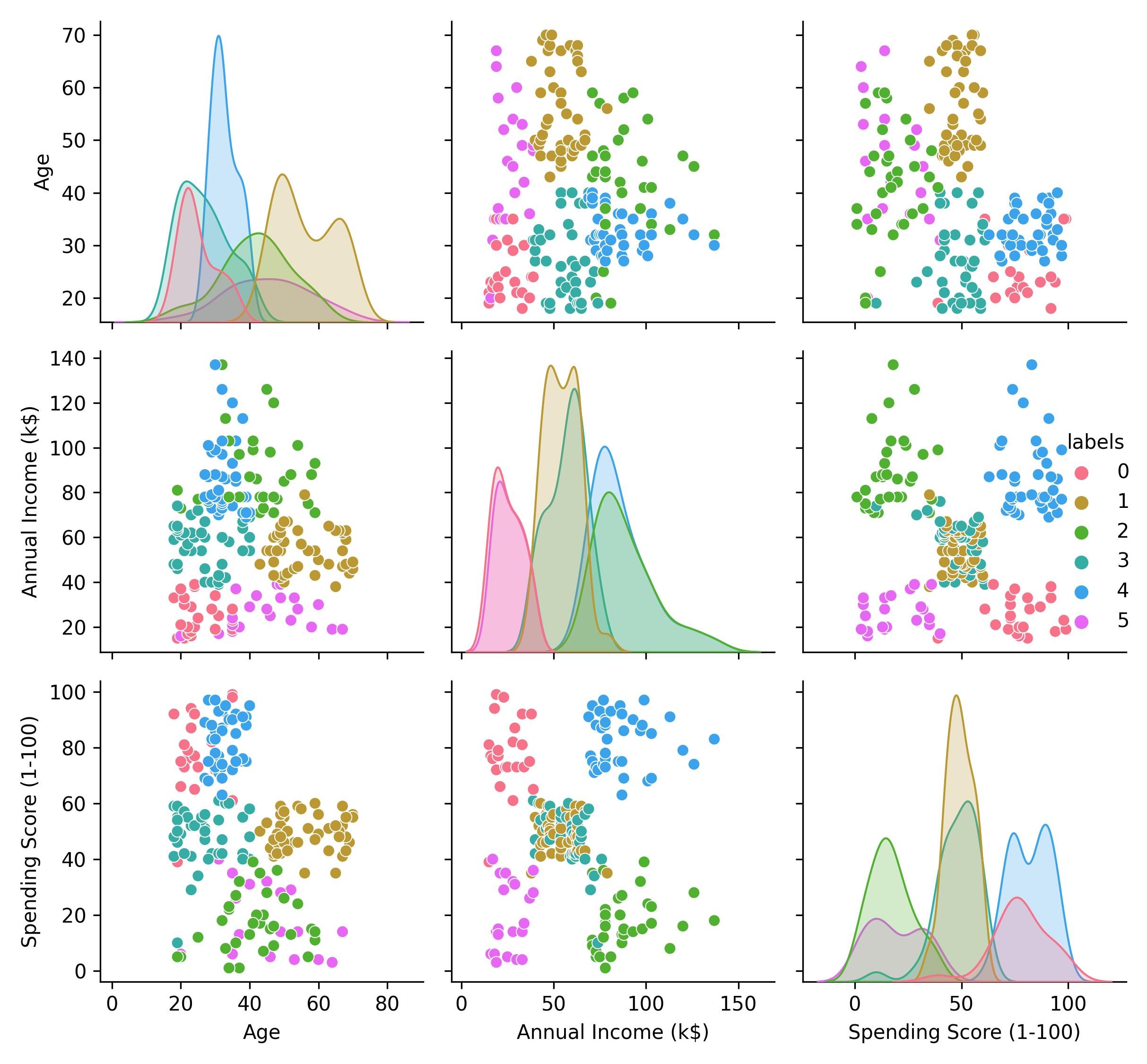
Clusters in the mall customers dataset.

• Cluster 0: lower income, higher spending score, 20-35 years old.

• Cluster 1: moderate income, moderate spending score, 40-70 years old.

• Cluster 2: higher income, lower spending score, 20-60 years old.

• Cluster 3: moderate income, moderate spending score, 20-40 years old.

• Cluster 4: higher income, higher spending score, 30-40 years old.

• Cluster 5: lower income, lower spending score, 20-65 years old.

From a business perspective, we could share these insights with the mall owners and invite them to consider some opportunities for additional customer research. For instance:

• Could the addition of affordable stores in the mall increase the spending activity of the individuals in cluster 5?

• Could the addition of high-end stores in the mall incentivize individuals in cluster 2 to spend more?

• If so, which kind stores?

The results of a cluster analysis are also useful to inform the design of marketing campaigns and high-level business decisions. For example:

• Does it make sense to expand business activities to previously unidentified groups of customers - such as clusters 2 and 5 in our example - based on the characteristics and sizes of the groups?

• If so, what marketing strategies would be most effective for these groups?

From an operational standpoint, it is often more practical to prefer coarser clustering structures (i.e., fewer clusters). This is one of the reasons why we favored 6 clusters instead of 10 or 11 in our example. In real-world applications, this approach can simplify the job of a Marketing team which might discover that - while distinct - some clusters might have the same response to certain marketing campaigns. Although a clustering algorithm may separate certain customers into different clusters, we might discover that these clusters can be treated as a single entity from a business perspective.

Limitations and Remarks

The tactics that we outlined have some limitations that are worth pointing out.

For density-based clustering algorithms such as DBSCAN, HDBSCAN, OPTICS, and other similar variants, scoring functions such as the Silhouette score, the Calinski-Harabasz score, or the Davies-Bouldin score should be used with care when we detect clusters that have non-convex shapes. In those situations, scoring functions that are less sensitive to the shape of the clusters - such as the Density-Based Clustering Validity index (DBCV) - are often preferred.

Furthermore, it is not always the case that scoring functions vary nicely as a function of the tunable parameters of a clustering algorithm. As in the example of the mall customers data, one can often identify more than a single optimal value for these parameters. One also needs to be careful about the fact that scoring functions do not automatically protect us from making foolish decisions such as selecting a trivial clustering structure. For example, this is what the full profile of the Calinski-Harabasz score looks like when we run k-means with very large values of k (the parameter that determines the number of clusters in k-means).

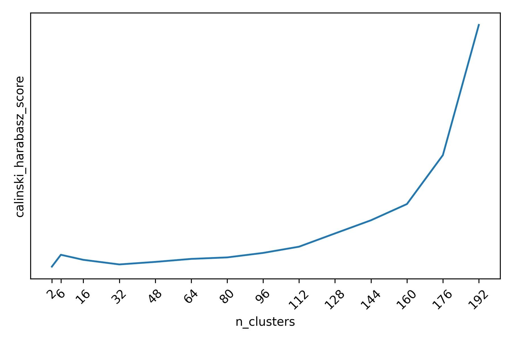
Calinski-Harabasz score for different k-means clusterings of the mall customers dataset. The score is maximized by a trivial clustering structure where each customer is a separate singleton cluster (k=200). However, the (local) maximum of interest is at k=6.

The Calinski-Harabasz score is maximized at the right boundary by the trivial clustering structure according to which every data point is itself a cluster. However, it is the local maximum at 6 the one that we care about.

Additionally, the computational cost associated with the tactics that we discussed can be high for very large datasets. This is because these tactics involve multiple runs to tune one or more clustering algorithms using different parameter values. The computational cost can be partially mitigated using Bayesian Optimization or other search optimization strategies instead of performing an exhaustive grid search.

Finally, our discussion was limited to clustering in the context of numeric variables and we measured similarity and dissimilarity between data points and clusters in terms of distances. However, the ideas that we discussed apply more generally.

Conclusion

In this post, we discussed 3 tactics that can be used to improve our chances of discovering meaningful clusters and being more confident about our discoveries. We showed that clustering algorithms can be tuned by means of sensible scoring functions. We also discussed that additional confidence about the final configuration of a clustering algorithm can be gained by evaluating the sensitivity of the tuning process to the choice of the scoring function: if multiple scoring functions lead to the same result, we are generally more confident about the validity of the clusters that the algorithm has found. Finally, we discussed that we can gain additional confidence about the clusters found by a particular algorithm if the same clusters are also found by other clustering algorithms.

Are you trying to extract meaningful insights from your data? Data Captains can help you!
Get in touch with us at info@datacaptains.com or schedule a free exploratory call.